Tutorial 9 - Sewer Design

This exercise will teach you how to complete the following sewer design tasks:

• Add a sewer data file to the project or create a new sewer data file.

• Import coordinate data containing node names, Y and X coordinates from an ASCII file.

• Change the display settings.

• Edit and set the link parameters.

• Edit the link tables.

• Input inflow data.

• Move existing nodes.

• Run the analysis and view the results.

• View quick long sections.

• Generate and view long sections.

• Calculate quantities according to SABS 1200.

• Set erf connection defaults and types.

• Graphically add erf connections.

• Run the erf connection analysis and view the results.

• Change the erf connection display settings.

• View the erf connection on the graphical vertical alignment.

• Generate a layout drawing with manhole names and a link schedule.

If you are continuing on from a previous tutorial, switch off all display options before you start.

If you haven't done so yet, read the Before You Start section before proceeding.

If you get lost or stuck while you are doing this tutorial, do one of the following:

• Press [Esc] to cancel all functions.

• Use File ► Open to re-open the same drawing and click No when prompted to save changes.

• Repeat the tutorial from the beginning, or from the last point where you saved the project.

Add a Sewer Data File to a Project

The first step is to create a new data file into which the sewer data will be imported. This file is added to the project file.

1. Load the Tutor drawing using File ► Open.

2. Change to Sewer mode by clicking the icon , or by selecting the Applications ► Sewer.

3. Add the water file to the project by selecting File ► Project Settings.

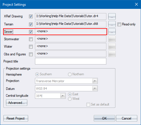
4. Select the Sewer checkbox and specify the name of the sewer file by clicking ... on the right, as shown above.

5. The file browser displays.

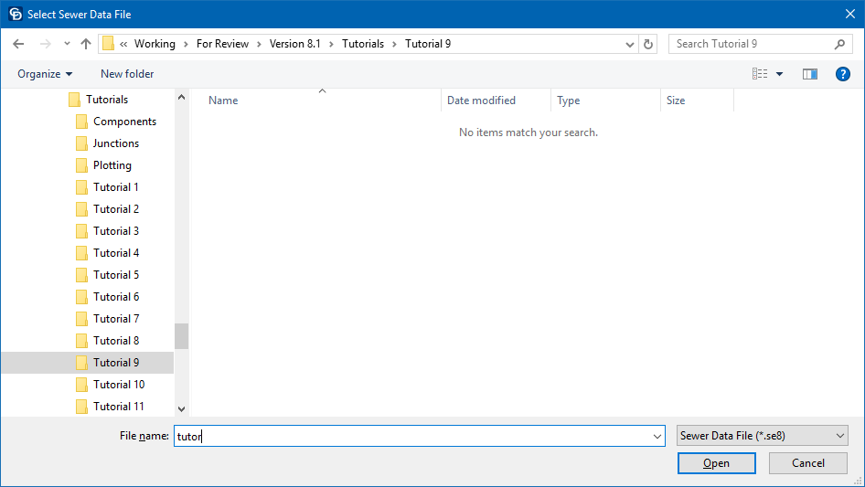
4. Navigate to a suitable subdirectory and find the existing sewer file, in this case 'Tutor.se8', and then click Open.

5. If you are creating a new file, you are asked if you want to create it.

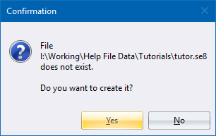
Click Yes to create the sewer file.

6. The Project Settings are updated.

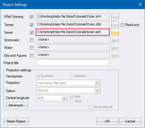
7. Click OK to proceed.

You have just created a new sewer project file, into which new data can be imported or typed.

Input Sewer Data

Data can be entered in a number of ways:

• Select Edit ► Node Data.

• Import an ASCII list of node coordinates.

• Import an ASCII file which includes the next node name, and link types and sizes.

• Load an existing layout drawing and classify it.

In this example you will import the manhole data from an ASCII file containing the manhole name, the next manhole name, Y coordinate and X coordinate for each manhole. The data items can be separated commas or spaces.

Import Coordinate Data from an ASCII File

1. Select File ► Import ► ASCII File.

2. The Import ASCII Data options display.

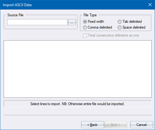
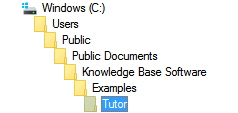
3. Click ... just to the right of the top edit control, and select the ASCII file 'SEWER.YXZ' from the Examples\Tutor folder.

4. The lines of the import file display.

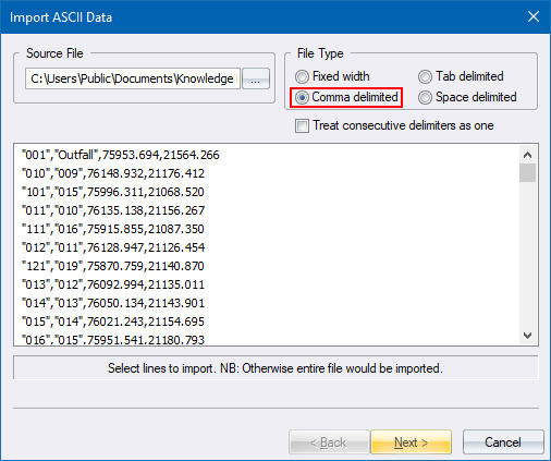
5. Select the Comma delimited option under the File Type section.

6. Now click Next to assign the file data to database fields.

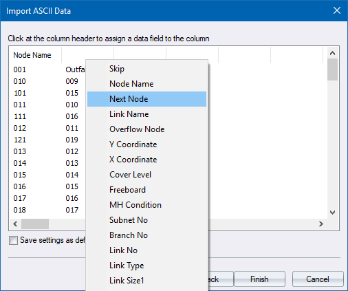
7. Click on the column headers to assign the column to a data field.

8. Specify the sequence of the column headers in the ASCII file as illustrated below - manhole (Node Name), downstream manhole (Next Node), the Y coordinate (Y Coordinate) and the X coordinate (X Coordinate).

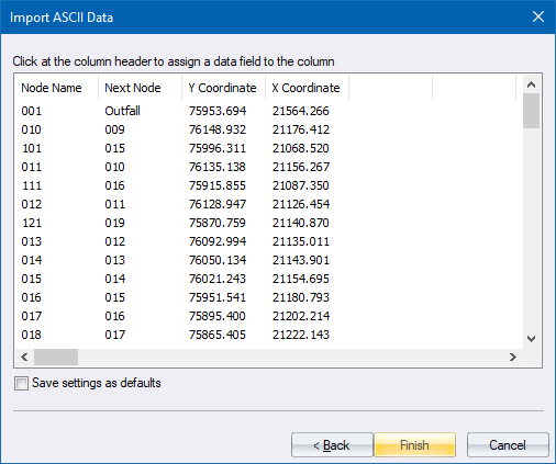
9. Click Finish to import the file into the newly created data file. The drawing is updated to display the imported sewer network.

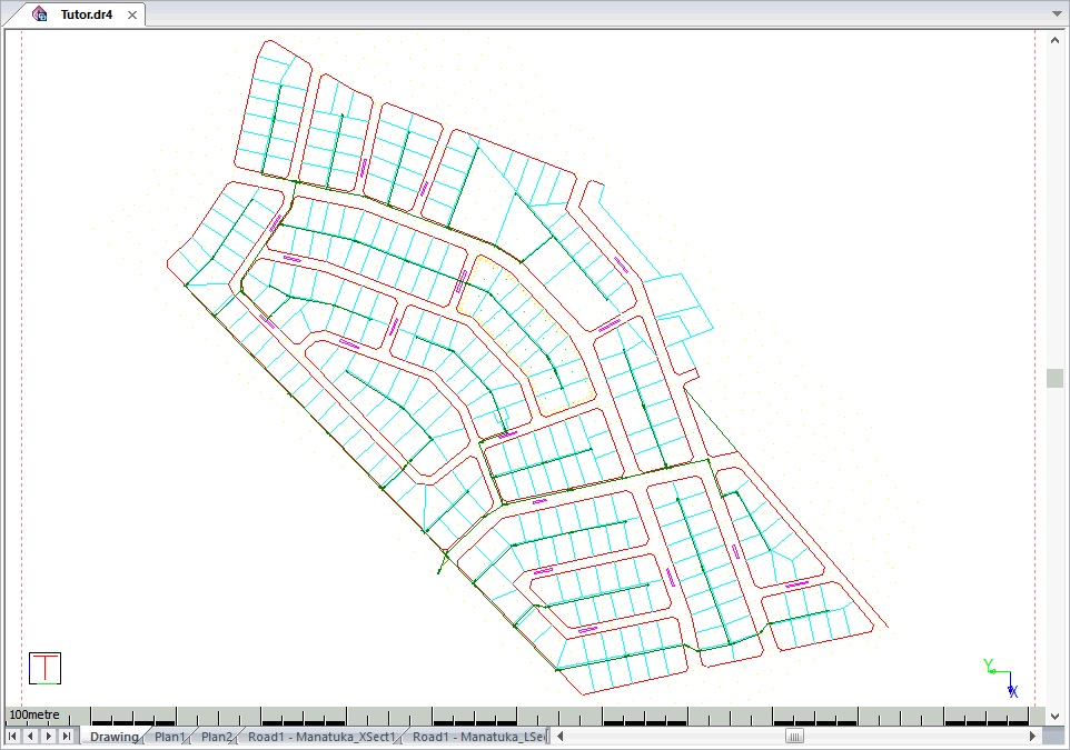
If you import data into an existing data file the program searches the existing data for matching node names and, if it finds an existing record, it update the fields in the record with the imported data.

Display the Nodes and Links

Civil Designer has many graphical functions to simplify the definition of nodes and links in the network. Obviously these functions can only be used if your data includes coordinates for the nodes.

1. Set up how the newly imported sewer data must be displayed by clicking on the Display Settings icon ,or by selecting Settings ► Display Settings.

You can specify how the data must be displayed and plotted.

2. Set up the Sewer section, as shown below.

Node Display Options

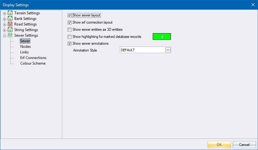
1. Click on the Nodes section.

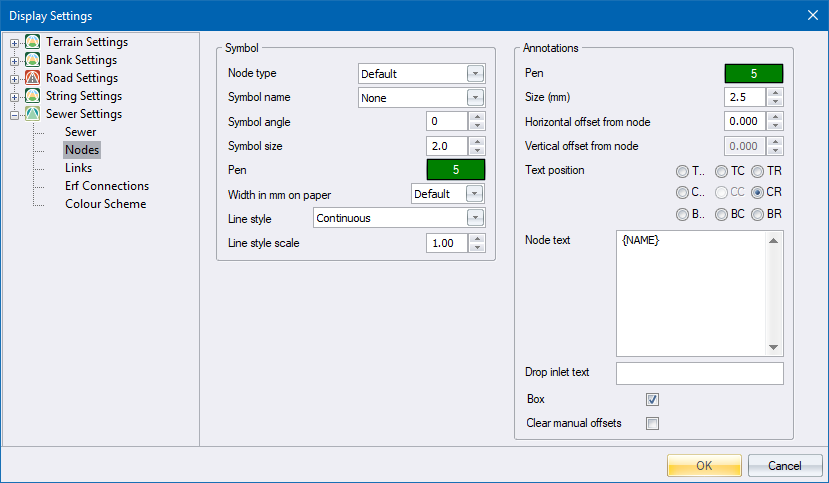
The Node settings allow you to define the pen, symbol size and line type for the node, the text pen and text size in points for the node annotations. as well as which annotations must be displayed.

2. In the Node text box, simply right-click and select the {NAME} option from the displayed list.

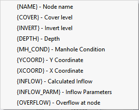
3. You can also add a pre or post-script to this text.

Links Display Options

1. Click on the Links section and the following displays.

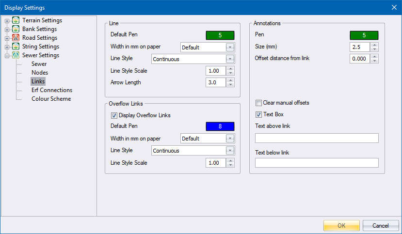
The Links settings allow you to define the pen, line thickness in mm and line type of the link display as well as the text pen and size in points for the link annotations, as well as which annotations must be displayed.

The Overflow Links settings allow you to define the pen, line thickness in mm and line type of the overflow link display.

2. Now you will change the display settings to show the link type and length at the midpoint of every link. You can specify which link attributes to display above and below the link in the Text above link and Text below link items.

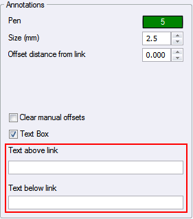
3. To define the text to be placed above the link, position the cursor in the edit control and right-click. A list of available attributes displays.

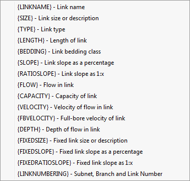
4. Select the {TYPE} option. The edit control is updated to display {TYPE}.

5. In a similar manner, add the text "{LENGTH} m" to the Text below link edit option. Note that the "m" must be typed in as it does not appear on the pop-up menu. Any combination of items selected from the pop-up menu and typed in can be made.

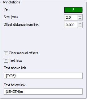
1. • You can vary the distance the link annotation is displayed from the link line, by changing the Offset distance from link setting.

   • If you want to add a box behind the link annotation, simply select the Text Box checkbox.

6. Set up the link annotations as shown above, and then click OK to update the display according to the settings you have just made.

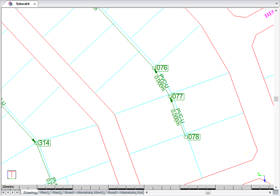
7. Position your cursor near a node and zoom in using the mouse wheel. The node name is displayed next to a circle representing the manhole. The link type is a default value for every pipe, in this case PVC-U, because the import did not specify a type. Note that the lengths are shown as 0.000m as these have not yet been entered or calculated.

Extracting Node Cover Levels from the Terrain Model

You will now extract node cover levels from the digital terrain model.

1. Select Graphical ► Cover Levels .

2. The following options display.

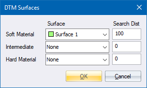
3. Here you specify from which terrain surface the cover levels must be interpolated. You can select any one of the 128 surfaces that contains valid data. The Intermediate and Hard Material settings are only used for quantity calculations.

4. Click OK. Civil Designer interpolates the cover level from the specified surface and replaces the current value.

5. To check the results, update the display settings to show the cover level next to each node. Select Settings ► Display Settings, or click the icon .

6. Position the cursor in the Node text box, and then right-click to access the list of available items.

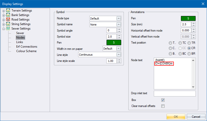
7. Type in 'CL=' and then right-click and select the {COVER} attribute. The entry should read 'CL={COVER}m'. as shown above.

8. Click OK. The display updates to display the node names, as well as the cover level at the node with the CL= prefix.

Set Node and Link Parameters

At this stage you have node data and connections, but have not yet specified link types and sizes. The node and link parameters have been set to the values and settings as set in the Defaults. These can be edited using Default Settings.

The easiest way to do this is to graphically select all the nodes and links, and then set the node and link parameters.

You will specify the link types, minimum cover and bedding class for the links. You can also specify the diameter or allow the analysis module to calculate the appropriate size.

1. Select Graphical ► Mark ► All to select the entire network. The selected links display in the specified highlight colour.

2. Select Tools ► Set Parameters to display the Set Parameters options.

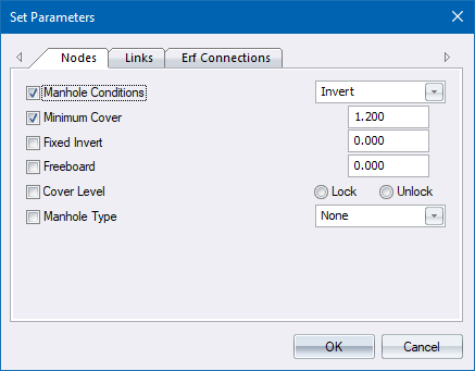
3. Set the following values for the nodes.

4. Set the following values for the links.

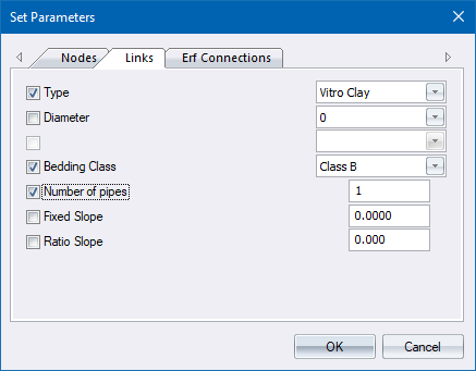
These settings set all links to be a Vitro Clay pipe on a Class B bedding. At the same time the nodes are set to have the inverts of the pipes common with a minimum cover of 1.2 m at the manholes.

5. Click OK to change the parameters.

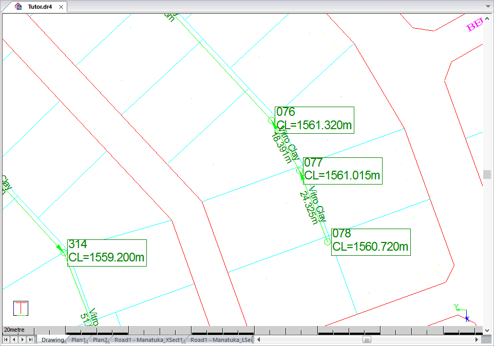
Notice that the link type text has been updated.

6. You can also change the link data of a selected branch. To do this first, select a branch by selecting Graphical ► Mark ► Upstream. This function selects a specific branch and all the incoming or upstream branches connected to it. Thereafter, follow the steps above with your required settings.

7. You can also change a single link by selecting Graphical ► Edit Data. Click on the node or link you want to edit in order to display the Data Editor for the selected node and link.

Edit the Link Tables

You want a minimum pipe size of 150mm in the network. Therefore, you need to go to the Link Table to view the available of the Vitro Clay link type.

1. Select Edit ► Link Tables ► Vitro Clay to display the Link Table, and then select Vitro Clay from the Link Table Selector list.

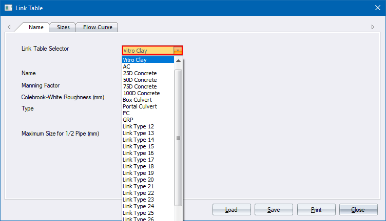
2. Now click on the Sizes tab. A list of available sizes for the Vitro Clay link type displays.

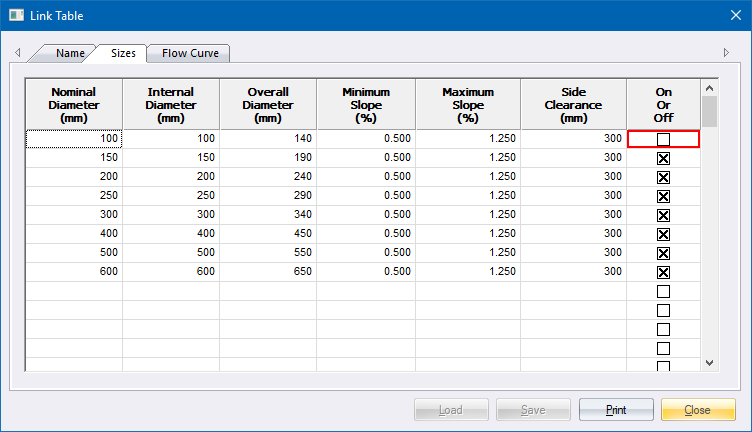
The smallest link size in the table is 100mm diameter, which you need to deactivate.

3. Select the checkbox in the On or Off column to deactivate the specific size.  The sizing then starts with the next active record.

4. Click Close to accept the changes.

Input Inflow Data

The inflow data must now be input for each node. The Sewer Module makes provision for Unit Flow, Harmon or Inflow Hydrograph inflows. This example uses Unit Flows so you must set the inflow method in the Design Parameters.

1. Select Edit ► Design Parameters.

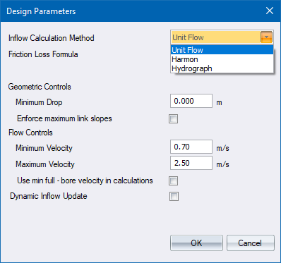
2. Set the Inflow Calculation Method as Unit Flow and click OK.

Inflow Classes

1. You can input up to five unit flow classes at a node. These classes are defined by selecting Edit ► Unit Flow Parameters.

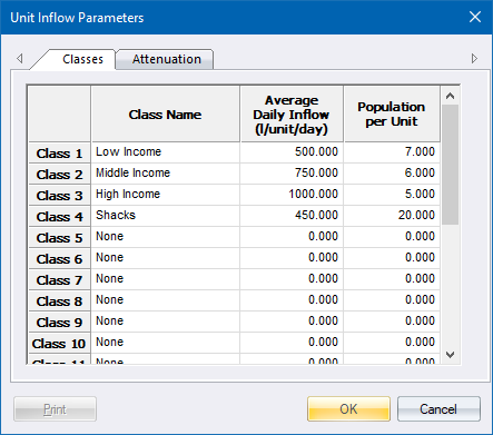
2. Now you need to add inflow classes to all your respective nodes. At present, the database is not itemised in any respective order. You first need to change the order of the records in the database so they follow in sequential order, making it easier for you to refer to and edit.

3. Change the order of the records in the data editors by selecting Settings ► Index Order. The Data Index options display.

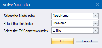
4. Select Node as the active node index and click OK.

5. Input the inflow data by selecting Edit ► Node Data menu option; or graphically by selecting Graphical ► Edit Data .

6. The Node Data Editor displays. Click on the Inflow tab to display the inflow settings.

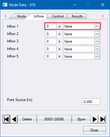
7. Select the required inflow class from the dropdown list and specify the number of units that contribute to this node.

8. Input the following Unit Flow inflows. Nodes with no inflows have been omitted.

9. Click Close when you have finished.

10. Alternatively you could use the data spreadsheet to input the inflows by selecting Edit ► Data Spreadsheet.

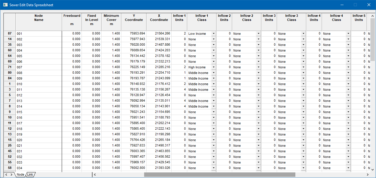
11. Close the spreadsheet.

12. Click Yes to save your changes.

Analyse the Network

At this stage you can analyse the network.

1. Select Analysis ► Network.

2. The program runs an error check on the data. If errors are found the error list displays. The listed errors must be corrected before the analysis can proceed. You can run the error check at any time by selecting Analysis ► Error Checking.

3. If no errors are detected the Analysis Parameters display.

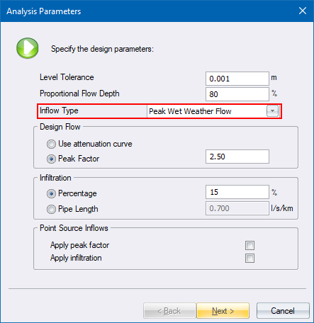
1. • The Level Tolerance option determines the accuracy that is applied in calculating the incoming and outgoing link levels in each node. Sometimes when you are evaluating an existing network with the links at fixed slopes, the rounding off of the slopes results in an incoming pipe which is, say 2mm, lower than the outgoing link that has been given a fixed inlet level. Normally, Civil Designer displays an error message in such an instance and then adjusts the inlet level of the outgoing link to be lower then the incoming link. This setting prevents the level adjustment if the difference is within the tolerance.

   • The Proportional Flow Depth determines the maximum flow depth that is allowed in the links. Usually a value of 80% is used.

   • You have a choice of 3 inflow categories in the Inflow Type list:

   • • Average Dry Weather Flow - Inflows based on unit flows only. No peak factor or infiltration.

     • Peak Dry Weather Flow - Inflows based on unit flow plus peak factor.

     • Peak Wet Weather Flow - Inflows based on unit flow plus peak factor plus infiltration.

Change the Inflow Type to Peak Wet Weather Flow.

1. • The Peak Factor is used in conjunction with the attenuation curve to calculate the attenuation at every node in the network.

   • The Infiltration defines the extra inflow due to stormwater infiltration as either a percentage or a fixed inflow value per km sewer pipe.

4. Set up the options as shown above and then click Next.

5. The general analysis options display.

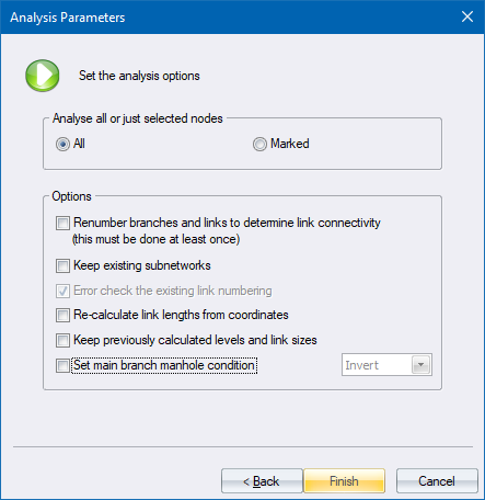
1. • These options allow you to specify whether you want to analyse all the nodes by clicking the All option, or just the selected nodes by clicking the Selected option, which allows you to select only a branch using Graphical ► Mark ► Upstream and then analyse just that portion of the network. You must however analyse the full network at least once before using this option.

   • If this is the first time you are analysing the entire network, (as is this case, you must select the Renumber branches and links checkbox.

   • The Recalculate link lengths from coordinates option calculates the length of each link from the coordinates of the upstream and downstream node coordinates. You must select this option as you  do not yet have link lengths.

6. Set up the page as shown above, and then click Finish. The Output Manager displays.

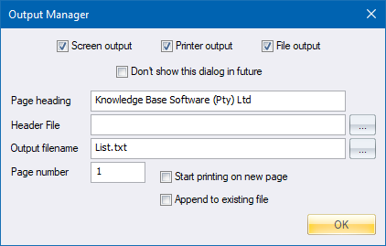
7. This allows you to specify the destination of the log that is generated during the analysis.

8. In this instance, direct the log to the Output bar by selecting the Screen output checkbox.

9. You are asked to confirm the branch and link re-numbering.

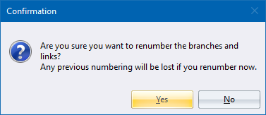
Click Yes to proceed.

10. When the analysis is complete, the results display.

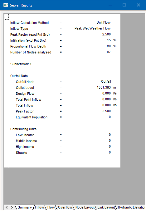
Each tab displays certain aspects of the results such as inflows, flows, overflows, levels and slopes, and hydraulic gradient.

Display Link Sizes and Slopes

You can now update the display settings to show the calculated link sizes and slopes.

1. Select Settings ► Display Settings or click the icon to set up the Sewer Link page, as shown below.

2. Take particular note of the Text above link and Text below link settings.

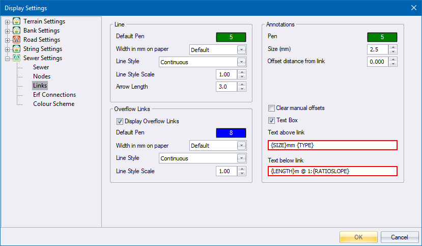
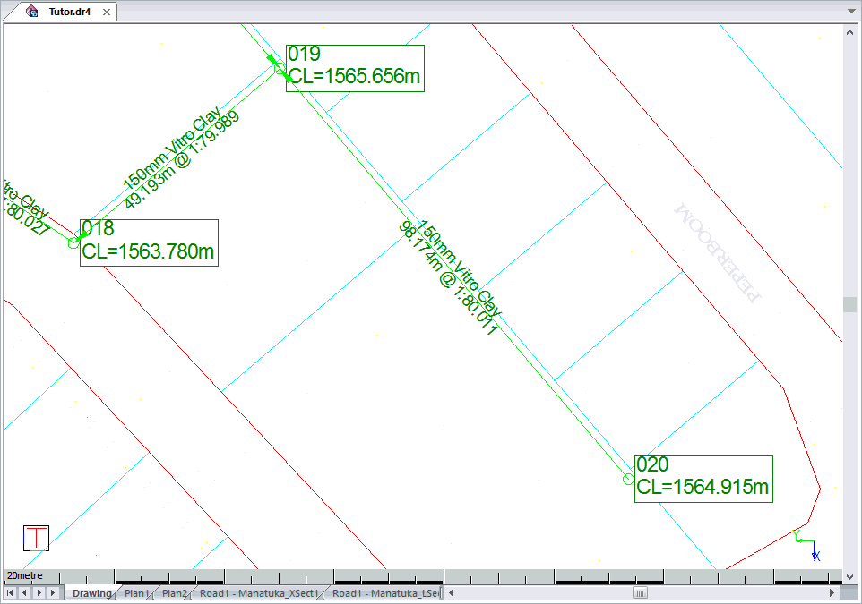
3. Insert {SIZE}, {TYPE}, {LENGTH} and {RATIOSLOPE} by right-clicking as previously described, and then inserting "mm" and "m @ 1: " manually.

4. Click Close to update the display.

Calculate Quantities

Quantities are calculated according to the parameters specified in the Bedding Class and Depth Increment settings.

These parameters can be changed from the Edit menu.

The quantity analysis is done on the selected links so you can calculate the quantities of the entire network, or just the selected links.

1. Select Graphical ► Mark ► All to select all the links in the network.

2. Select Analysis ► Quantities.

3. After the analysis, the quantities display in a series of tables. Each table contains the results of a particular quantity calculation.

Erf Connections

Sewer also analyse erf connections, and even allows you to automatically adjust the level of the main sewer network to try and accommodate the erf connections that cannot tie into the network.

Erf Connection Defaults

1. Select Erf Connections ► Erf Connection Defaults, or click the icon in the toolbar.

2.  The Erf Connection Defaults display.

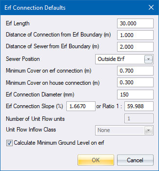
Set the values as shown above. The settings are for erf connections that connect onto a mid-block sewer for the erven adjacent to the sewer servitude.

The connections will be inside the erf 1m from the erf boundary, and the main sewer is positioned outside the erf in an adjacent erf 2m from the erf boundary.

3. Click OK to accept the settings.

4. Select Erf Connections ► Erf Connection Types. The Erf Connection Types display.

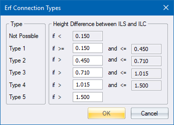
Set the depth increment envelopes as shown above.

If the difference between the invert level of the main sewer line (ILS) and the invert level of the erf connection (ILC) is less than 0.15m, the connection is not possible.

The type of connection depend on the height difference envelopes that have been specified.

Add Erf Connections

You will enter the erf connections between sewer nodes 205 and 204, which are situated in the bottom right corner of the site.

Switch the site contours on in the display settings to see the slopes on the erven.

First, enter the erf connections that are situated on the northern side of the sewer line. Therefore the erven where the sewer is outside the erf as defined by the Outside Erf option in the Erf Connection Defaults.

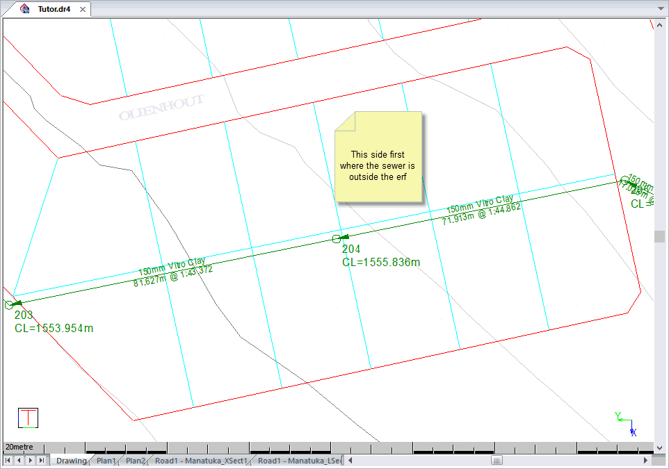
1. Select Erf Connections ► Add Erf Connection, or click the icon to enter the erf connections.

2. You are prompted to:

Add Erf Connection: Indicate position on correct side of sewer link: Height = 1556.996

3. Indicate the position of the new erf connection. You can use any of the snap modes to do so. As the cursor moves ,the elevations are interpolated from the selected soft material DTM surface and displayed in the prompt area.

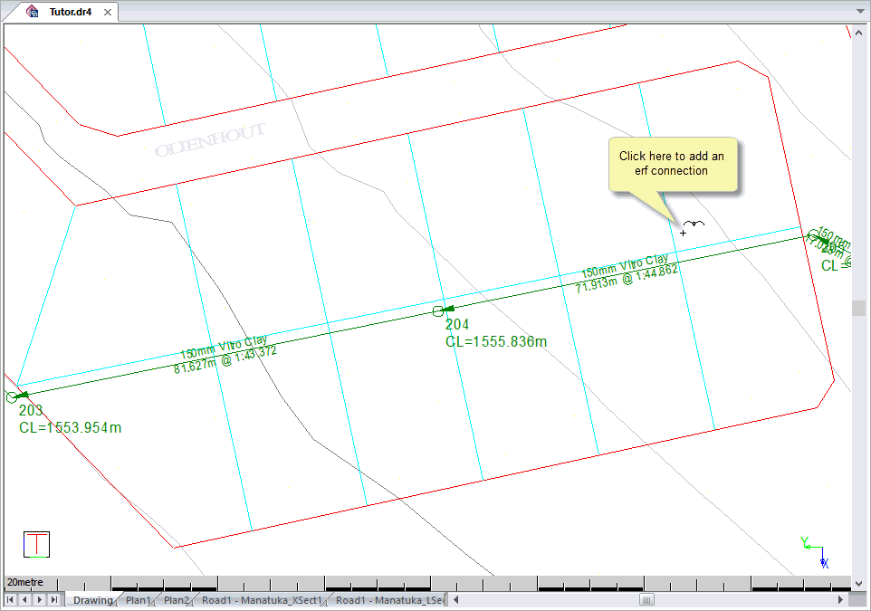
4. Once you have clicked pressed [Enter] at the desired position, you are prompted to:

5. Type in a new erf connection name, e.g. 10011 and press [Enter] or click Enter.

6. If the Calculate Minimum Ground Level on Erf option is selected in the Erf Connection Defaults, you are prompted to:

MGL: Indicate erf for minimum ground level calculation (right click for options)

7. Click in the middle of the polygon that defines the erf perimeter for which you are adding the erf connection.

8. The program traces the drawing lines that form the erf boundary around the selected erf, and then search for the lowest point inside the erf. The drawing elements forming the erf boundary must be a closed polygon for this function to work.

9. The minimum ground level (MGL) is extracted from the soft material DTM surface and the Erf Connection Data Editor displays.

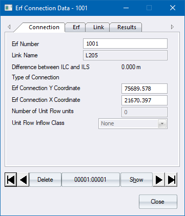
The following data is calculated and entered by the program from the erf connection defaults, sewer network and the dtm:

1. • Node Name

   • Erf Connection Y Coordinate

   • Erf Connection X Coordinate

   • Erf Length

   • Distance of Sewer from Erf Boundary

   • Sewer Position

   • Ground Level at Erf Connection (GLC)

   • Minimum Cover on Erf Connection

   • Minimum Cover on House Connection

   • Erf Connection Slope as Percentage or Ratio

   • Erf Connection Diameter

   • Link Length

   • Link Slope

   • Node Invert Level

   • Distance from Node

   • Link Y Coordinate

   • Link X Coordinate

10. Activate the display of the newly created erf connection by clicking the Display Settings icon or selecting Settings ► Display Settings.

11. Select the Show erf connection layout checkbox and then click  the Erf Connections sub-item in the Sewer section.

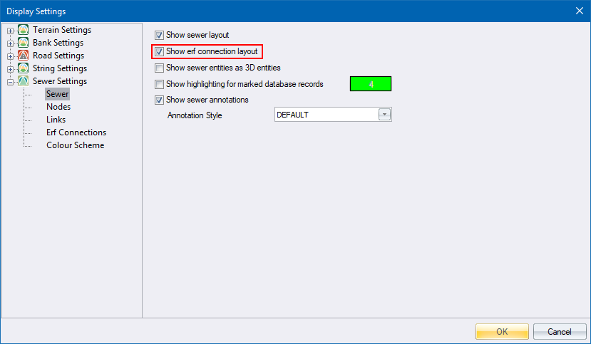
The Erf Connections settings allow you to define the pen, line width and line type for the erf connection, the text pen, text size in points and text placement settings for the erf connection annotations, as well as which annotations must be displayed.

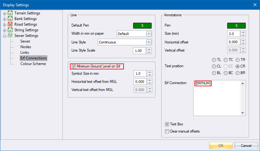
The Minimum Ground Level on Erf option specifies that the symbol indicating the lowest point on the erf is drawn together with the height level.

12. Change the settings as shown above, and then click OK. The erf connection is drawn, as shown below.

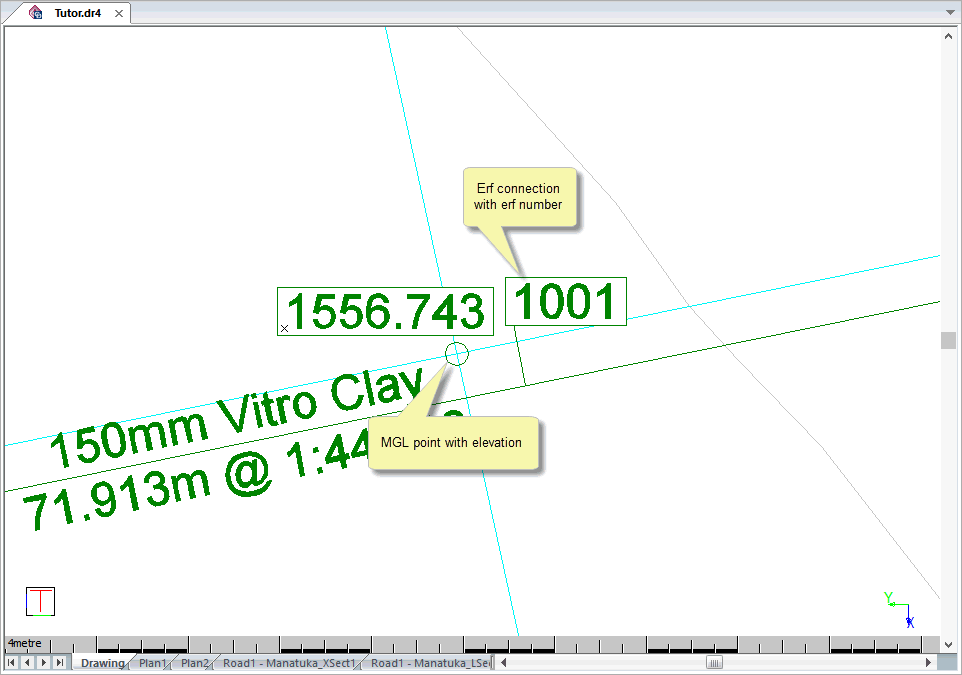
13. You are prompted to:

Add Erf Connection: Indicate position on correct side of sewer link: Height = 1556.996

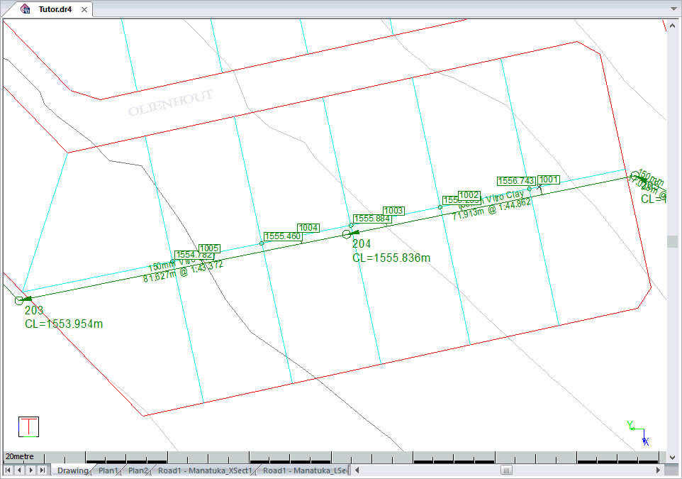
14. Continue to add the other five erven on the northern side of the sewer line.

15. Press [ESC] to terminate the function.

16. Now change the erf connection default settings to enter the erf connections where the sewer line falls inside the erven.

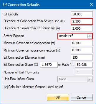
Set the Sewer Position as Inside Erf. Set the Distance of Connection from Sewer Line value to 2.3m, but remember this is now the distance from the sewer line that the erf connection is situated.

17. Click OK to proceed.

18. Add the erf connections on the southern side of the sewer link in the same manner as above.

Analyse Erf Connections

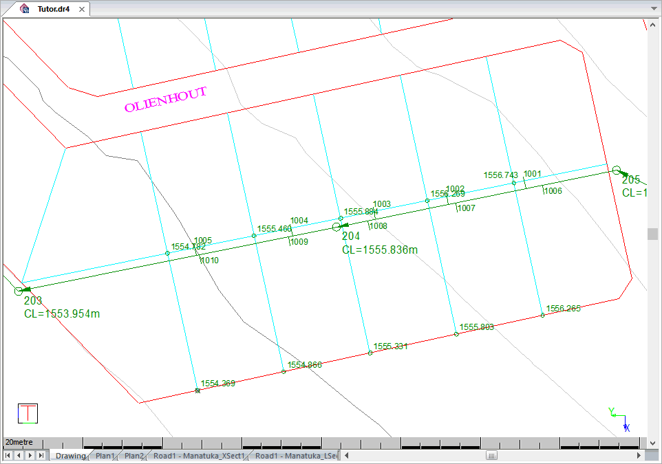
Erf Connections are calculated according to the parameters specified in the Erf Connection Data and Erf Connection Types settings.

These parameters can be changed from the Edit menu.

1. Select Erf Connections ► Analyze Erf Connections.

2. After the analysis the erf connection results display.

You can see that you have a problem since in the Type of Connection column only 5 erven are Type 1 and the rest are Not possible.

This means that only five erven can drain to the main sewer line. The rest are too deep to connect to the main sewer line.

You therefore need to lower the main sewer line.

3. Close the Erf Connection Results.

4. You can view the erf connections on your graphical longitudinal section, and visually lower the required manholes. Select Tools ► Vertical Alignment to display the Vertical Alignment Editor.

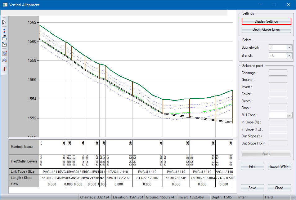
5. Click Display Settings to display the display options for the Long Section Editor.

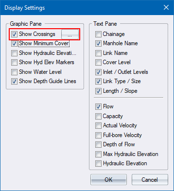
6. Select the Show Crossings checkbox  to display the Crossing Services list.

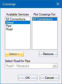
7. Select the Erf Connections entry in the list on the left and then click Select. The Erf Connections is now listed on the right-hand list.

8. Click OK to continue, and then click OK again to close the Display Settings for the long section.

9. The Vertical Alignment Editor displays the long section with the erf connections, as shown below. Use the mouse wheel to zoom in on the area where the erf connections are.

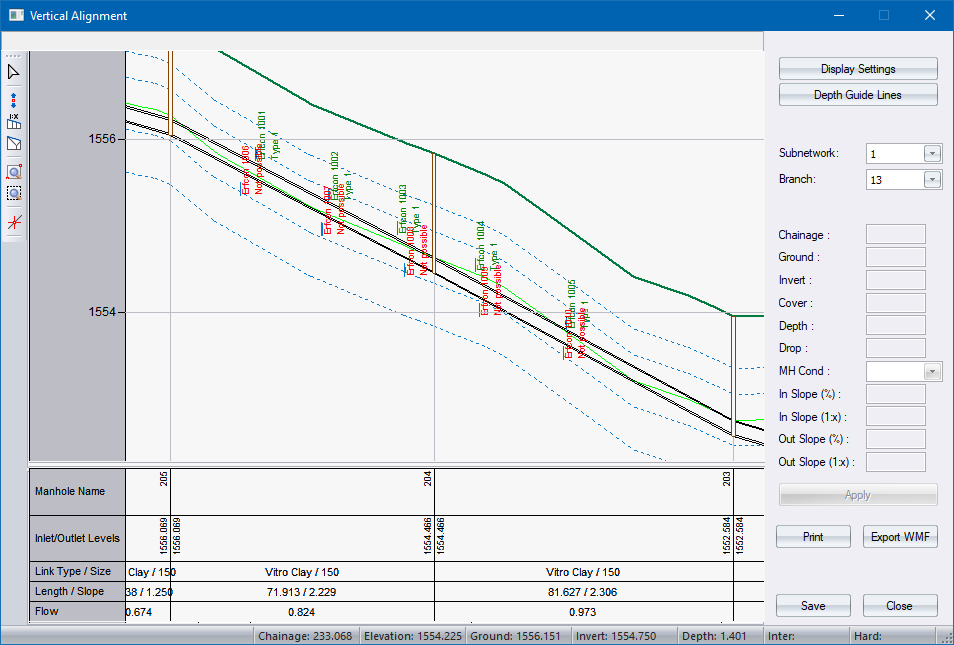
The erf connections that have been connected to the sewer line display in green. Those that cannot be connected display in red.

10. You want to lower the sewer line from node 205 to 203 so the red erf connections can be connected successfully. Click on the Invert Adjust icon on the toolbar on the left of the Long Section Editor. Now click on manhole 204 as shown below.

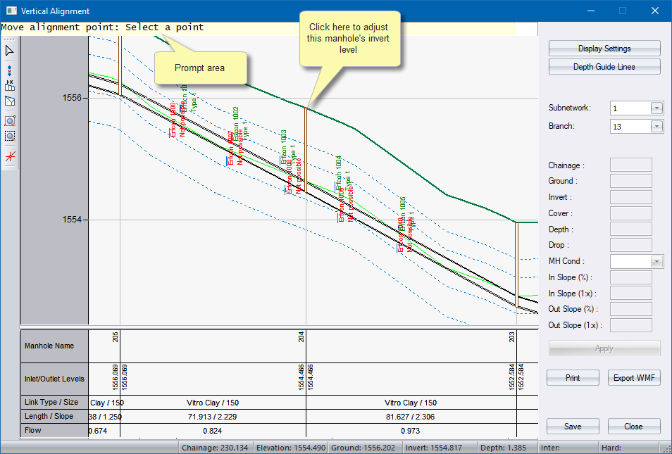
11. Simply drag the bottom of node 204 lower until the link between 204 and 203 runs below the red erf connections as shown below. Then click to fix the level.

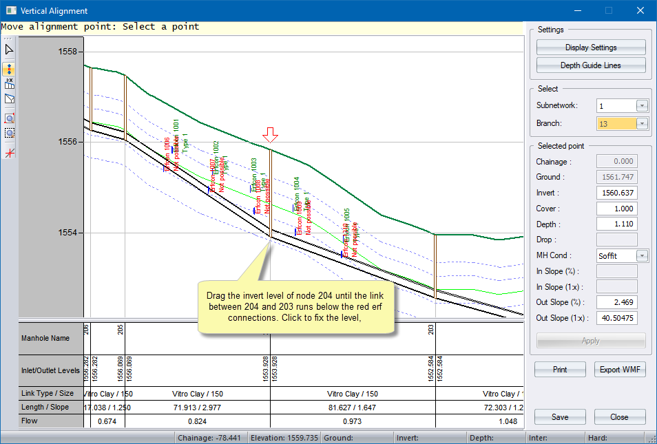
12. You can see that erfcon 1006 to the left is still not able to connect, so lower manhole 205 in the same way until you have something similar to the long section below.

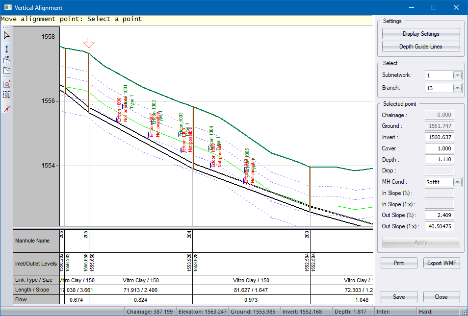
The sewer pipes must pass below the incoming erf connections.

13. Click Close and then click Yes to save your changes.

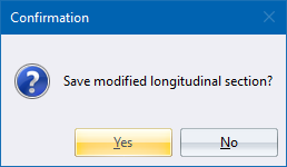
14. Now you need to analyse your sewer network again to incorporate the above changes. Then, also analyse the erf connections to see what the influence is on the erf connections.

All the erf connections now can drain successfully to the main sewer line.

Printing Input Data and Results

At this stage you may want to produce a hard copy of the design. This is done with the Print Settings, which output selected data items to a printer or an ASCII file.

1. From the Sewer menu select File ► Print Sewer Data.

2. The Print Settings display. Select the data items you want and the output device, as shown below.

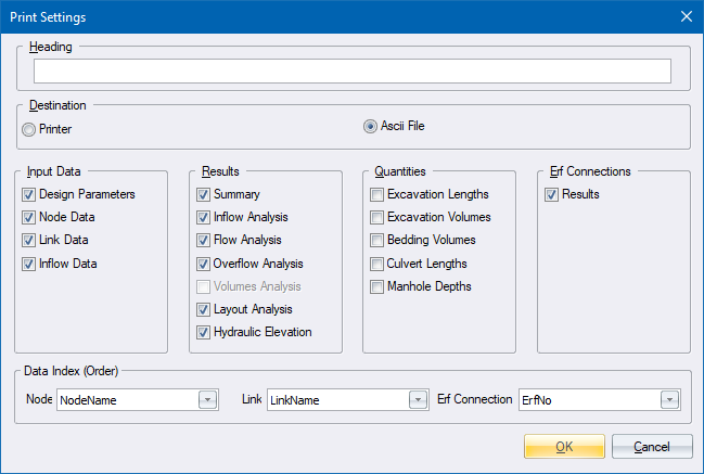
3. Click OK to start printing.

Creating the Final Layout Plan

Now that the design is complete, it is time to update the original cadastral drawing with the sewer layout, along with a coordinate list and a link schedule.

1.  Select Plot ► Generate,or click the icon .

2. The Plot Setup displays.

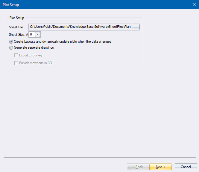
3. Use the same sheet file you used in the earlier tutorials, namely Shared Documents \Knowledge Base Software\Sheet files\Plan.sht.

4. Click Next to continue.

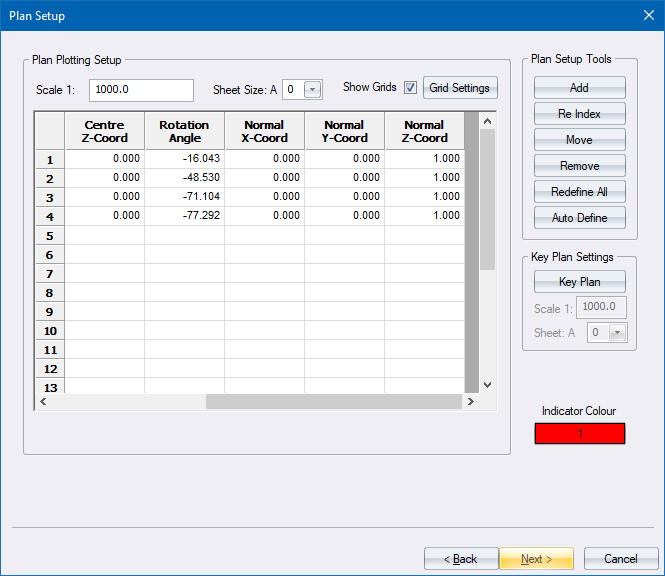
5. Accept the Plan Setup options as they are, and then click Next.

6. The Plan Lists options display.

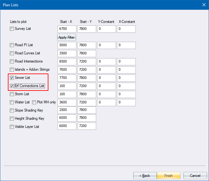
7. Check the Sewer List and Erf Connections List options as shown above, and then click Finish to generate the plan.

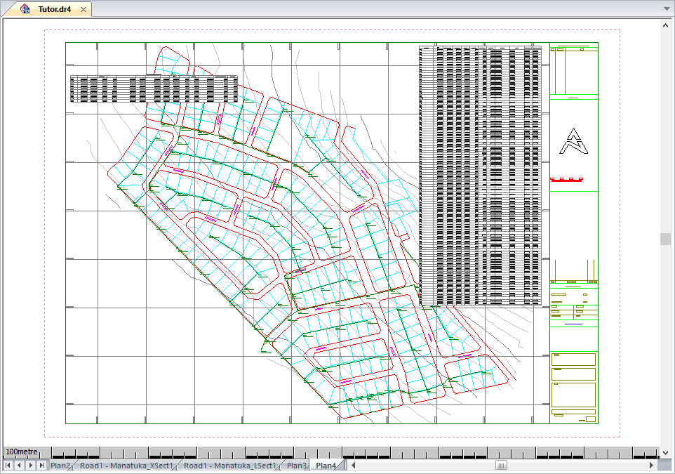
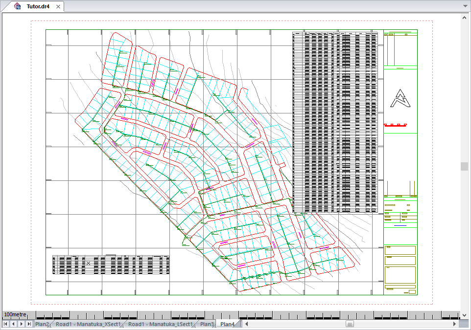
8. Click and drag to move the Erf Connection schedule from the top left of the drawing to the bottom left.

Plotting Sewer Long Sections

1. Select Plot ► Generate, or click the icon .

2. This time, select the Sewer Longsection sheet and set the sheet size to A0.

3. Click Next to display the long section plot setup.

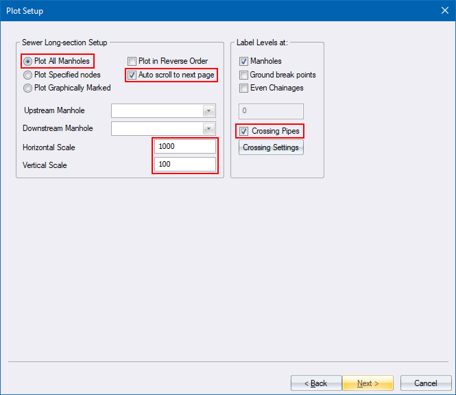
4. Specify the Horizontal and Vertical scales as 1:1000 and 1:100 respectively. Also specify that all manholes must be plotted and to scroll to the next page.

5. Click Next.

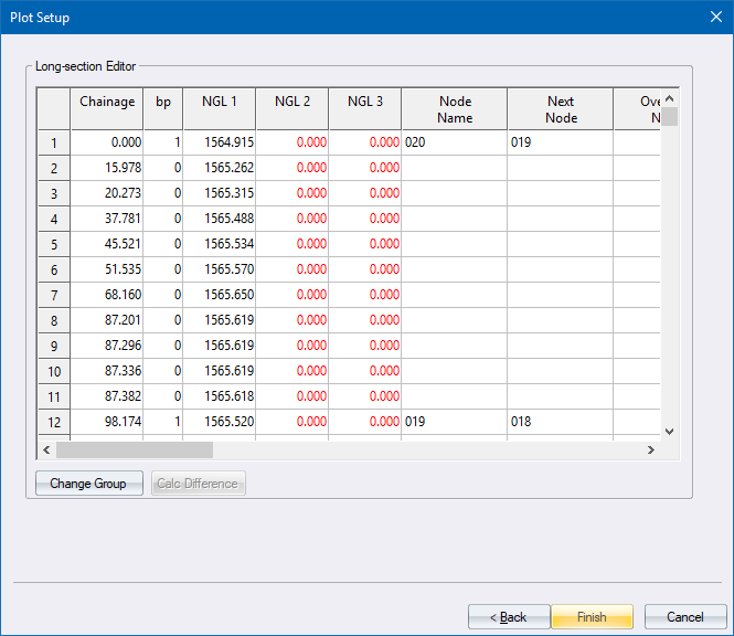
You have the option to edit long section data, if required.

6. Click Finish to create the sewer longsection layouts. You selected the Auto scroll to next page option so multiple layouts are created until all the sewer pipes have been plotted.

Save Your Design

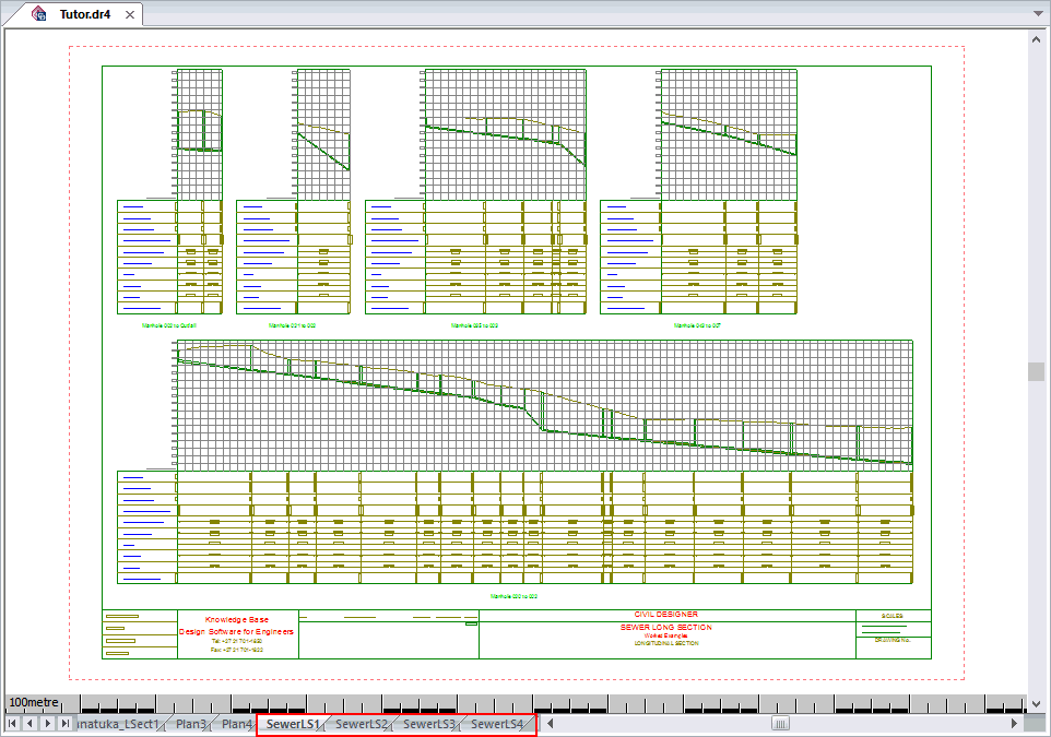
You have now completed Tutorial 9.

You can now:

• Experiment on your own.

• Exit the program using File ► Exit.

• Go on to one of the other tutorials Tutorial 10 - Storm Design,or Tutorial 11 - Water Design.