If
you would like to use a different screen background colour, you can change
the Drawing background colour using Settings
► View Settings.
If
you would like to use a different screen background colour, you can change
the Drawing background colour using Settings
► View Settings.In order to familiarise yourself with the Water Mode, it is advisable to complete the following tutorial.
This tutorial will teach you how to:
Add a water data set to an existing project.
Change the water network display settings.
Modify features in the water model.
Analyse the network.
View results in various formats.
View databases.
Plot long sections.
The first step is to create a new water data file into which the water data will be imported. This water data file is added to the project files in the Project Settings dialog. You need to attach the "Tutor with EC.wdf" water data file to the project.
If you have already worked through any of the previous tutorials, you can open and continue working with your existing Tutor project. You would then only need to attach the water data file.
If you have not yet worked with the Tutor project, you will first need to open the "TUTOR.dr4" drawing file. In this case, load the Tutor drawing by selecting File ► Open and navigating to the "Users\Public\Public Documents\Knowledge Base Software\Examples\Tutor" folder. Open the "TUTOR.dr4" file.
If
you would like to use a different screen background colour, you can change
the Drawing background colour using Settings
► View Settings.
For those starting the project from scratch, you need to add the "Tutor.dt8" terrain file to the project in the Project Settings. To do this, change to Survey mode and select File ► Project Settings. Select the Terrain checkbox and click ... (Browse). Navigate to the "C:\Users\Public\Public Documents\Knowledge Base Software\Examples\Tutor" folder and open the "Tutor.dt8" file.
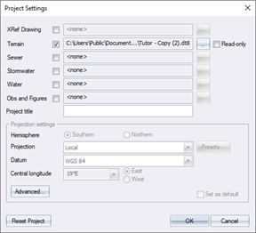
The file has already had the survey data imported into it and the model has been triangulated.
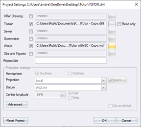
For this Water project, you will need to attach the "Tutor with EC.wdf" water data file to the project in the Project Settings. To do this:
Add the water file to the project by selecting File ► Project Settings.
For this tutorial, you will be using an existing water file so click the checkbox next to Water. Click ...(Browse) and navigate to "C:\Users\Public\Public Documents\Knowledge Base Software\Examples\Tutor" . Select the existing water file found in the folder, in this case "Tutor with EC.wdf" and click Open.
In practice,
when you don't have an existing file to work with, you will follow the
same procedure of checking the relevant design file box in the Project
Settings and browsing for a folder in which to save the file. You then
need to give the file a name. The program will tell you this file doesn't
exist and ask if you want to create it. Click Yes.
Once the project file has been created, ensure you are in Water mode by selecting Applications ► Water Mode.
In this tutorial, you have linked an existing water file to the project under File ► Project Settings for the network data.
Generally, when setting up a water model the network data can be read into Civil Designer in various ways, namely:
Import Civil Designer 6.x Project files.
Convert Drawing/CAD entities to a network.
Import Wadiso files.
Import Epanet.
Import LandXML.
Import Text File.
Use the Water Graphical interface to generate your network.
See the
Data Preparation section in the
Help File for more detail on preparing a CAD drawing for conversion to
a Water network.
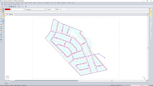
Your loaded water model layout should look similar to below.
When using the Convert drawing entities option to create a water model from a CAD drawing of the network layout, it is important to remember that if your drawing does not contain information such as pipe diameters or demands, Water will assign the default settings (as set in the Settings ► Pipe Defaults and Settings ► Node Defaults) to the network on importing.
These default Pipe and Node settings are also assigned to the water nodes and pipes when using the Graphical menu options to draw in your nodes and pipes.
For this tutorial, you are working with an existing water file and, as such, there is no need to change the Node and Pipe default settings.
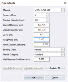
Material - uPVC - SABS 966
Pressure Class - 9
Nominal Diameter - 110
Cover - 900mm
Roughness - 0.100mm
Minor Losses Coefficient - 2.00
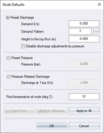
For this tutorial, the existing Water file you attached to your project already had the water property connections added to it and, as such, you already have the projects demands assigned to the water network. Therefore, there is no need to add demand to the Nodes.
If, however, you are creating a new water model by converting CAD entities, you could add the demands for each node as text onto one separate layer and have these demands assigned to each node in the network when converting from CAD.
Alternatively, you can add your demands by drawing in your house connections graphically or have Civil Designer add house connections automatically by making use of the new parcel functionality.
If you
need clarity on what information needs to be set in a dialog, press [F1]
while the dialog is open to launch the Civil Designer help file for that
particular dialog.
In the Node Defaults, the Preset Discharge setting is used to set the demand at each node.
The Preset Pressure setting is used to model inflow into a network.
Click OK to close the dialog.
Furthermore, you can use Graphical ► Edit to graphically select which entity you would like to edit.
Once your water network is set up, you may find your network features are not immediately visible.
To activate the display of the Water module, click the Display Settings icon or select Settings ► Display Settings. The Display Settings dialog displays, allowing you to specify how the data displays and plots.
Set up the display for each Water network feature by selecting the relevant page and changing each default setting to suit.
Right-click inside the Annotation Text boxes to view and select from the automated text data items that are available. You can add your own text where necessary.
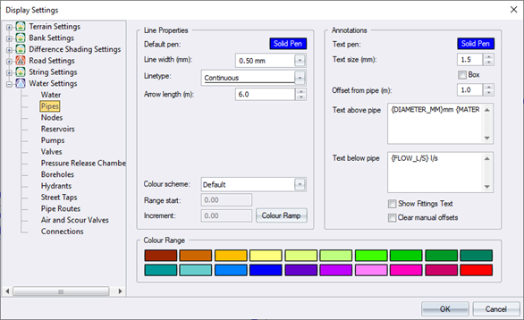
Similarly, the nodes and reservoir settings can be edited to suit. Once you have set up the required settings, click OK. The Water network displays with the new settings.
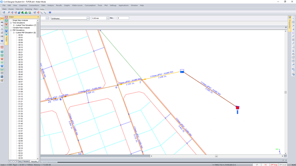
Position your cursor near a pipe and zoom in using the mouse wheel, the [Z] key to display the zoom menu, or [M] or [D] to magnify or de-magnify to see the new display settings. Your display will look similar to the image below.
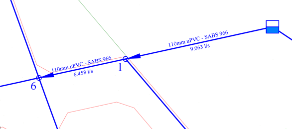
The model shows the pipe diameter and pipe material, as well as the flow in l/s. You might need to first analyse the network to view the updated flow values.
You will
change the display settings again after running the analysis to view the
various results.
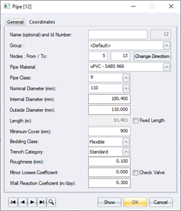
At this stage, you will look at the existing model and modify it where necessary before you do an analysis.
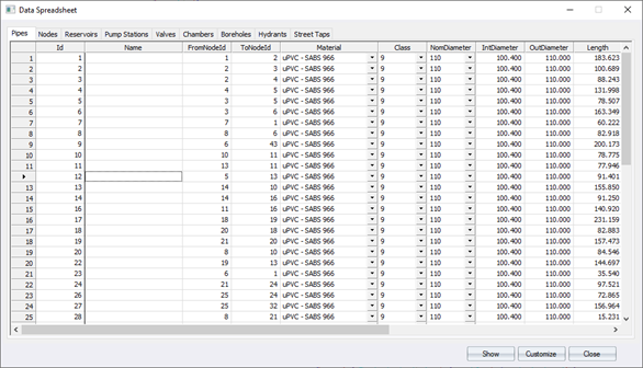
Select Data ► Summary.
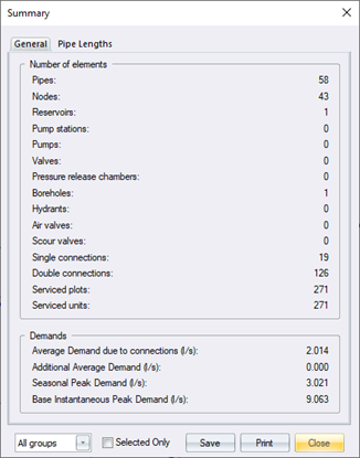
From the summary, you can see that there are 58 pipes, 43 nodes and 1 reservoir in the network in total.
The average demand of the network is 2.014 l/s. Since you have applied various demand patterns to the nodal demands, you have a Seasonal Peak Demand of 3.021 l/s and an Instantaneous Peak Demand of 9.063 l/s.
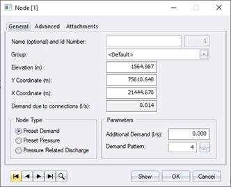
The Tutorial network is a portion of a larger network. It is not necessary to model the entire system in Water, as you are able to model the inflow from an adjoining system by defining the inflow at the relevant node. In this case, node ID number 73 is feeding the network via a borehole, but this could have been an incoming pipe from an adjoining network.
 .
.
The Find Record window displays.
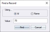
Select the Id radio button and type “73” in the Value field.
Click Find and the program displays information for node 73.
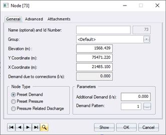
As mentioned
earlier, you could have modelled the inflow from this node as a Preset
Pressure but for this tutorial project you are using the latest borehole
functionality available in Civil Designer.
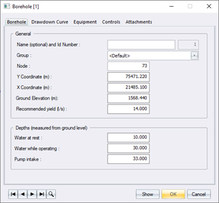
The water while at rest and while operating, and Pump intake depths are measured from ground level and have already been set from the data collected from the Hydrological report. To view the pump details, select the Equipment tab. For this tutorial, the borehole pump has already been selected.
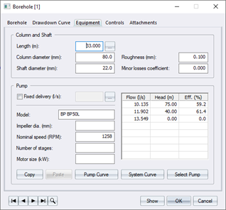
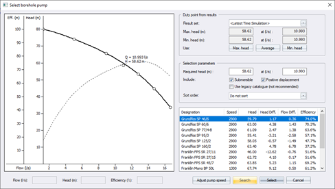
If, however, you need to select a pump, you can click Select Pump and search for a pump meeting the requirements.
For this tutorial, use the preselected Mono BP 50L positive displacement borehole pump. You do, however, need to check that the level controls for your borehole pump are set up correctly to switch the pump on and off based on water levels in the reservoir.
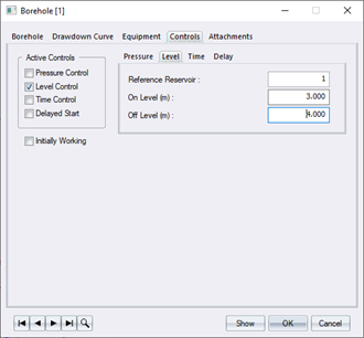
Select the Controls tab in the Borehole dialog and ensure the Level Control box is selected and the Level Settings are set in the Level tab, as below. You are switching the pump on when the reservoir water level drops to a depth of 3m. Also ensure the Initially working option is unchecked.
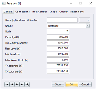
You will now edit the Reservoir capacity and elevations, as well as set the initial water depth in the reservoir, which is used at the start of the analysis.
You can either select Data ► Reservoirs, or use one of the other selection methods.
You also need to set the incoming and outgoing pipes for the reservoir. To do this, select the Connections tab.
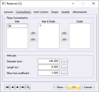
To check which pipe is the Inlet and Outlet at the reservoir, select to show the pipe ID number in the pipe Display Settings.
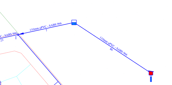
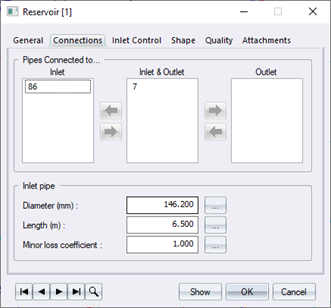
The pipes connected to the reservoir are listed in the Inlet & Outlet section. Select the correct pipe number to activate the "move arrows". Click on the arrow to move the selected pipe to the Inlet or Outlet section.
Water allows flow in one direction only, so it is not necessary to define a non-return valve on the pipe, unless you want to introduce a control valve i.e. modulating or on/off valve.
The error check looks at the basics of your model, i.e. are your nodes all connected to a pipe, have you specified pipe diameters, do you have a draw off somewhere on your network, is there at least one head in your network to allow for an analysis, etc.
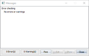
There should be no errors in your model. However, if there is an error message it will inform you where the problem lies so you can fix it.
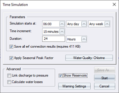
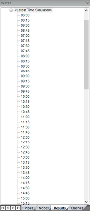
A time increment less than 15 minutes is not recommended since the demand pattern factors are defined every 15 minutes, making anything less senseless.
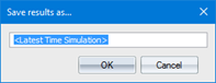
As a default, the analysis is saved as '<Latest Time Simulation>'.
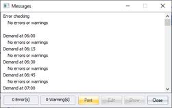
You have an option to:
Click Print to print the errors.
Click Show to view the problem item.
You can view the results in many ways.

Similarly, you can set up the desired settings for the nodes, reservoirs, boreholes, etc. Click OK to close.
The colour schemes can indicate problem areas visually, while the displayed text indicates the actual flows in the pipes.
Select the Flow column header to sort the flows from highest to lowest. In this way, you can pick up critical flows in the system.
You can view the pipes with the critical flows by highlighting the line and clicking Show.
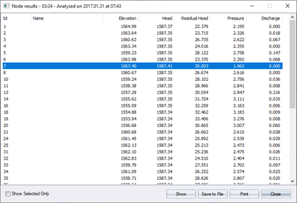
Click Close to close the Results tables.
Close the Results Browser window.
Select Graphs ► Pipes to open the graphical display of the results of each pipe.
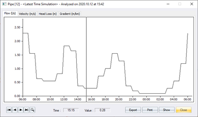
Use the arrow buttons to browse between the various pipes. From the pipe results table, you determined the critical pipes.
In the graphical display, once at the critical pipe, you can select the most critical period visually. It is not practical to view, print or save results of the entire 24 hour simulation at every 15 minute interval. You would normally require about two to three outputs, i.e. period of the lowest and highest demands/flows/pressures and possibly an average value.
You can click Print to print the graphs.
You can view the graphical results for the other network features in a similar manner.
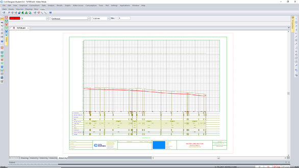
The Water long section plot requires you to select the desired pipes for plotting. You can select the pipes to plot graphically, or create Pipe Routes from one selected node to another. These pipe routes become available for selection when running the plot routine.
Once you
have selected the pipes, the process is identical to that of the Sewer
or Storm modules.
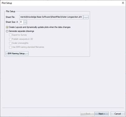
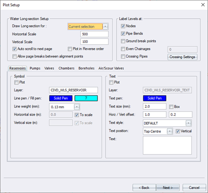
Select the various elements you want visible in your long section and then click Next.
Click Finish.
You can plot multiple layouts that dynamically update as you make changes to your model. Below is an example of a Water long section plot.